Comparing two independent groups
[1]:
import os
import pandas as pd
import matplotlib.pyplot as plt
import numpy as np
import math
import scipy.stats

age_shf = pd.read_pickle("../data/processed/age_shf")
age_ebn = pd.read_pickle("../data/processed/age_ebn")
We’ve looked at correlation, which quantifies how much one variable is related to another variable of the same individual, for example height and weight, or income and expenditure on food. When it’s necessary to compare different groups, for example the height of men and height of women, we use different tests:
- the parametric \(t\)–test, and
- the non–parametric Mann–Whitney U test
These tests work by comparing the means to see if they are statistically significantly different. Obviously the means of different samples will be different, so how much they differ before we conclude they are statistically different depends on the variance of the groups.
\(t\)–test
The independent samples \(t\)–test is used when comparing two independent groups, such as the heights of a group of males and the heights of a group of females. We have a sample of males and measure their heights, and a sample of females and measure their heights. Crucially the height of one respondent does not affect the height of another respondent, so the measurements are independent. The level of measurement of both groups should be continuous (numerical interval or ratio) and we are comparing the same variable (height).
For our example we have ages of two groups: people from Sheffield and people from Eastbourne. We saw in an earlier section on standard errors and confidence intervals that their means were different, and the confidence intervals suggested the population means were different also:
[2]:
age_shf.C_AGE_NAME.mean()
[2]:
37.87209832494418
[3]:
age_ebn.C_AGE_NAME.mean()
[3]:
42.83316903391945
The measurements are independent (i.e. the age of people in Sheffield does not affect the age of people in Eastbourne) and continuous (numerical) so we can use an independent samples \(t\)–test to statistically test if the means are different:
[4]:
scipy.stats.ttest_ind(
    age_shf.C_AGE_NAME, age_ebn.C_AGE_NAME, equal_var = False
)
[4]:
Ttest_indResult(statistic=-58.84359690127882, pvalue=0.0)
The \(p\) value is \(<< 0.01\) so we can reject the null hypothesis that there is no difference between the ages of people in Sheffield and the ages of people in Eastbourne (i.e. there is a difference in mean age). In this case this is not surprising because we actually have two populations, but this is intended to be illustrative only.
Assumptions
As always, there are assumptions. We have met the assumption of independent observations and the variable (age) is continuous, so these assumptions were met. The \(t\)–test also assumes that if the sample sizes are small they should be normally distributed, but this is not relevant in our case. If you need to test for this, plot a QQ plot:
[5]:
scipy.stats.probplot(age_ebn.C_AGE_NAME, plot = plt)
[5]:
((array([-4.3447271 , -4.14589489, -4.03774648, ...,  4.03774648,
          4.14589489,  4.3447271 ]),
  array([  0,   0,   0, ..., 100, 100, 100])),
 (24.361214673692874, 42.833169033919454, 0.9854839451271551))
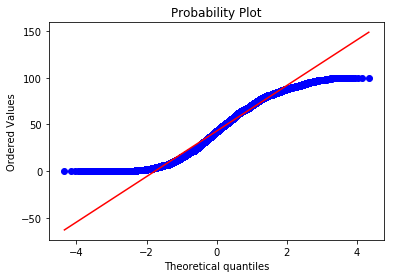
[6]:
scipy.stats.probplot(age_shf.C_AGE_NAME, plot = plt)
[6]:
((array([-4.70745961, -4.52329906, -4.423601  , ...,  4.423601  ,
          4.52329906,  4.70745961]),
  array([  0,   0,   0, ..., 100, 100, 100])),
 (22.700384057589815, 37.872098324944176, 0.9846609326125065))
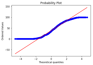
These are not normally distributed (if they were the blue points would lie along the red line), but this doesn’t matter in this case because we do not have small samples. We also need to check that the variances of the two groups are approximately equal using a Levene’s test:
[7]:
scipy.stats.levene(
    age_shf.C_AGE_NAME, age_ebn.C_AGE_NAME
)
[7]:
LeveneResult(statistic=1358.0920464422002, pvalue=5.4491601311285835e-297)
Ah. The \(p\) value is highly statistically significant, so we should reject the null that the variances are not different (i.e. there are). In this case we should use values adjusted to correct for unequal variances (this is actually the default behaviour for scipy.stats.ttest_ind()):
[8]:
scipy.stats.ttest_ind(
    age_shf.C_AGE_NAME, age_ebn.C_AGE_NAME, equal_var = False
)
[8]:
Ttest_indResult(statistic=-58.84359690127882, pvalue=0.0)
If the variances were approximately equal the \(p\) value would be \(> 0.05\) and we would not reject the null. If this were the case we could perform an equal variances \(t\)–test, by specifying equal_var = True.
Mann–Whitney U
The Mann–Whitney U test is a non–parametric version of the \(t\)–test useful when we do not have continuous data (but the variable should be at least ordinal) or we otherwise violate one or more of the assumptions of the \(t\)–test. It stil assumes that the measurements are independent.
Mann–Whitney U works by ranking the observations without considering the groups they’re from. If there was no difference between groups the sum of the ranks would be approximately equal. If there is a difference between groups the sum of the ranks for each group will differ. Using our example age data:
[9]:
scipy.stats.mannwhitneyu(
    age_shf.C_AGE_NAME, age_ebn.C_AGE_NAME
)
[9]:
MannwhitneyuResult(statistic=24316208190.5, pvalue=0.0)
And reassuringly we can see the statistic is statistically significant. We wouldn’t really use a Mann–Whitney U test for age (continuous) data; this is just to demonstrate the syntax and interpretation. Mann–Whitney U tests are useful in the social sciences though because we deal with ordinal data (e.g. Likert scales) a lot.
Dependent groups
The \(t\)–test and Mann–Whitney U test assume that the observations are independent. In our example the two groups are independent because the age of people in Sheffield does not affect the age of people in Eastbourne.
There are situations when the observations are dependent and these tests are not appropriate for this type of data. In the social sciences, this is common with longitudinal data (data where the same individuals are asked a survey at different points in time). Such repeated measures data is not independent.
In these cases we can test for differences in means, but I’m not going to go into how to do this here; there are plenty of resources to help. I’m bringing this up here so that you are mindful of the test(s) you use if you have repeated measures or longitudinal data.