Central tendency

import pandas as pd
import matplotlib.pyplot as plt
import numpy as np
import math
import scipy.stats

food = pd.read_pickle("../data/processed/food")

One of the first things we usually want to do is to explore and describe our data, before we begin any detailed analysis. Measures of central tendency are one of the first things we use to describe our data.

Measures of central tendency is a fancy phrase for ‘average’. They are a single data point used to represent a ‘typical’ value from your data. Depending on your level of measurement you can use one or more measures of central tendency.

Mode

The most common value. Mode is the only measure of central tendency you can provide for nominal data.

For example, the variable A121r in our food data set is of household tenure type. The available options are:

1. public rented (i.e. rented from a council)
2. private rented (i.e. rented from a landlord)
3. owned

A frequency (count) table of this variable shows that owned is the most common type of tenure:

food["A121r"] = food["A121r"].astype("category")
food["A121r"].cat.categories = ["public rented", "private rented", "owned"]
food["A121r"].value_counts()

owned             2777
public rented      864
private rented     715
Name: A121r, dtype: int64

Median

The median is the ‘middle’ point. It’s only appropriate for ordered data (i.e. ordinal or numeric) and is calculated by arranging your data in order and selecting the mid–point. P344pr is the gross normal weekly household income for each respondent. The following are incomes for the first five respondents as an example:

food["P344pr"].head()

0    465.36
1    855.26
2    160.96
3    656.22
4    398.80
Name: P344pr, dtype: float64

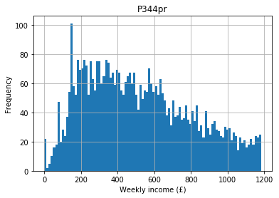
The variable looks like this when we plot it as a distribution:

food.hist("P344pr", bins = 100)
plt.xlabel("Weekly income (£)")
plt.ylabel("Frequency")

Text(0, 0.5, 'Frequency')

If we arrange these in order and take the middle point we obtain the median income:

food["P344pr"].median()

476.799

If your data have an even number of items, the median is the mean (average) of the two middle points. For example, using the following example data with four data points - 2, 4, 6, 8 - there is no one middle point. Instead 4 and 6 are the middle points. The median is the mean of these, which is \(\frac{(4 + 6)}{2} = 5\).

The median is often considered more robust than the mean, which means it is less susceptible to outliers, for reasons we’ll get to in a moment.

Mean

The mean is what most people think of when they think of an average. You simply “add them all up and divide by how many you have”. For example, the mean of the incomes is:

food.P344pr.mean()

518.3056177244473

If the incomes were an ideal normal distribution, the mean and the median (and mode) would be identical (more on the normal distribution later). In the wild, most distributions are not exactly normal (or ideal) so the mean and the median differ, as we have seen with our example data.

If there are outliers in our data set these can affect the mean up or down. For example, if there are a few individuals in our data that are substantially wealthier than most this can affect the mean. They also affect the median, but not as much as the mean. For this reason we often consider the median a more robust measure of central tendency than the mean, and why you should be careful when someone presents a mean value without any additional information.