Data sources

Software

To be able to analyse your data you are first going to need to enter your data into your computer, in a software programme of your choice. Software for statistical and quantitative data include SPSS, R, Python (usually with Pandas), and Stata. Even Excel can be used for descriptive statistics and some basic analysis with additional modules!

These pages focus on Python (specifically Python 3), but statistical and quantitative analysis is software–agnostic, and the principles here can be used with any software. Many beginners prefer SPSS because it is easier to get started with, but it is still powerful enough to do almost all analyses.

Data structure

Regardless of which software you choose to use, you will need to enter your data in the same format. Each row should correspond to one individual, and each column to one variable. This is often called long form. Here’s an example of what a data table might look like:

id	age	sex	preferred hot drink
1	36	m	coffee
2	44	f	tea
3	52	m	hot chocolate

Each row represents a person (person 1, 2, or 3) and each column represents a piece of information about that person, or a variable. Here we have age (a number), sex (male or female), and their preferred hot drink. Reading across the top row, we can see that person 1 is aged 36, is male, and prefers coffee.

Secondary data (data that someone else has collected) will usually come in this form, and it is good practice to enter our primary data (data we collect) in this form too. To enter the above example data into a spreadsheet would look like this:

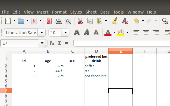
This can then be saved and entered into our analysis programme of choice.

Tutorial data

These tutorials use a number of teaching data sets available from the UK Data Service and Nomisweb (FYI Nomisweb have a great API for reproducible research) under terms of the Open Government License:

Office for National Statistics, University of Manchester, Cathie Marsh Institute for Social Research (CMIST), UK Data Service, 2016, Living Costs and Food Survey, 2013: Unrestricted Access Teaching Dataset, [data collection], Office for National Statistics, 2nd Edition, Office for National Statistics, [original data producer(s)]. Accessed 1 October 2018. SN: 7932, http://doi.org/10.5255/UKDA-SN-7932-2. Contains public sector information licensed under the Open Government Licence v2.0

Office for National Statistics, 2014, 2011 Census. Accessed October 2018. Contains public sector information licensed under the Open Government Licence v2.0.

The census data contains information about areas, rather than people, so areas are the individual unit of observation. The food dataset contains information about individual people.

If you’re following along at home I download and process the data sets with scripts in the src/ directory.

%run ../src/01-download.py

The food dataset (Living costs and food survey) includes income, but this is top–coded. For the purpose of these exercises I simply remove the top–coded cases to make the distributions a bit more normal. If you were analysing this data for real you would need to consider how to handle these top–coded cases.

%run ../src/02-process.py